
The pivot table in a spreadsheet is used to summarize the data set for analysis purposes. It converts the vast data set into tabular form, which is simple to understand. Pivot tables can be used to view the data set from several aspects. In addition, using the provided suggestions, one can make pivot tables for the first time. Let’s look at how to make pivot tables in a few easy steps.
1. Select the set of data
The data for air conditioners sales in North and South India are there in screenshot 1.The divisions are further divided into different states in North and South India, and for each product, information on the units sold and the price per unit is provided.
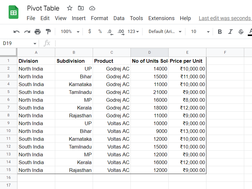 Screenshot 1: Our initial data set
Select the data set you wish to turn into a tabular format ; in this case, we are picking A1 through E15. By selecting the entire data set, a pivot table will be built around it.
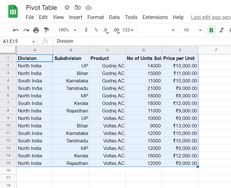 Screenshot 2: Select data
2. Inserting the pivot table
Once the data set has been chosen, click on Insert to bring up the drop-down menu where you may choose a pivot table. Click on Pivot to proceed to the next panel, and screenshot 3 is provided for reference.
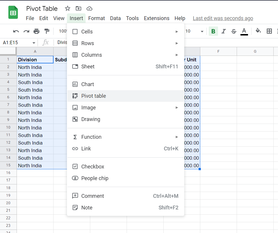 Screenshot 3: Insert Pivot table
When you choose Pivot Table, a new panel displaying Create Pivot Table in New Sheet appears on screenshot 4. Select Create Form here to continue to the table area.
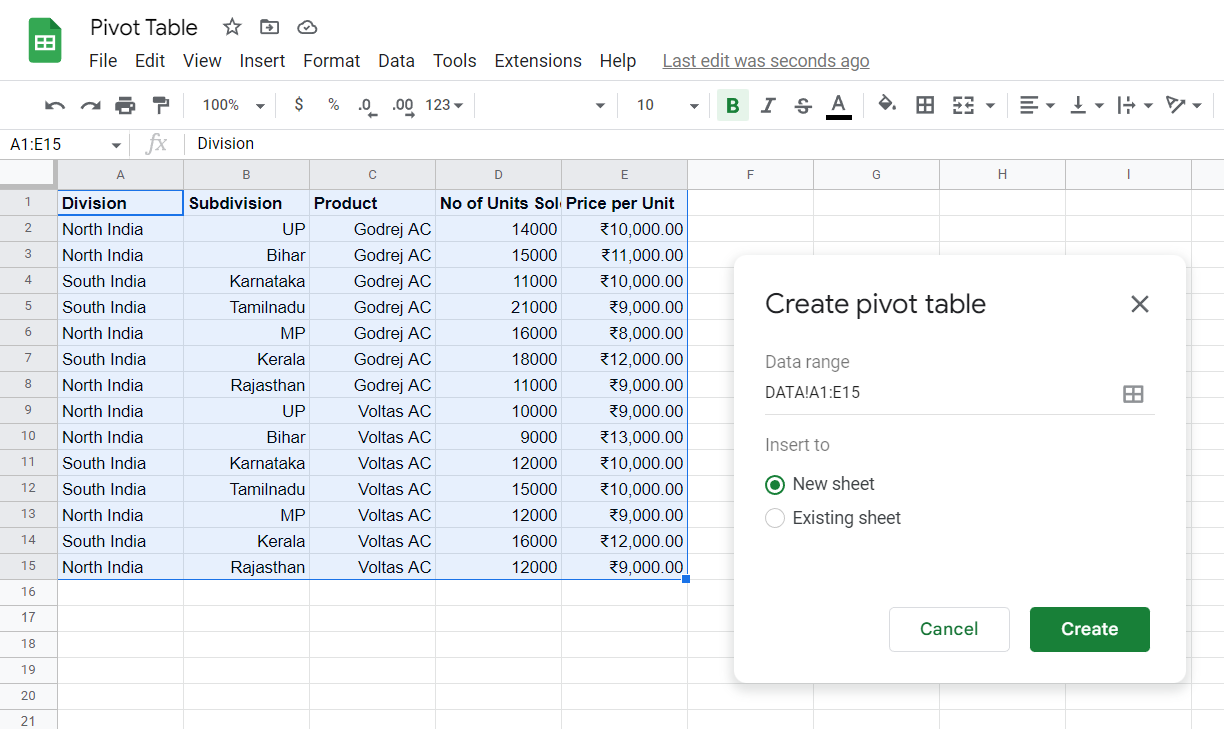 Screenshot 4: Select “New sheet”
3. Obtain a table from suggestions
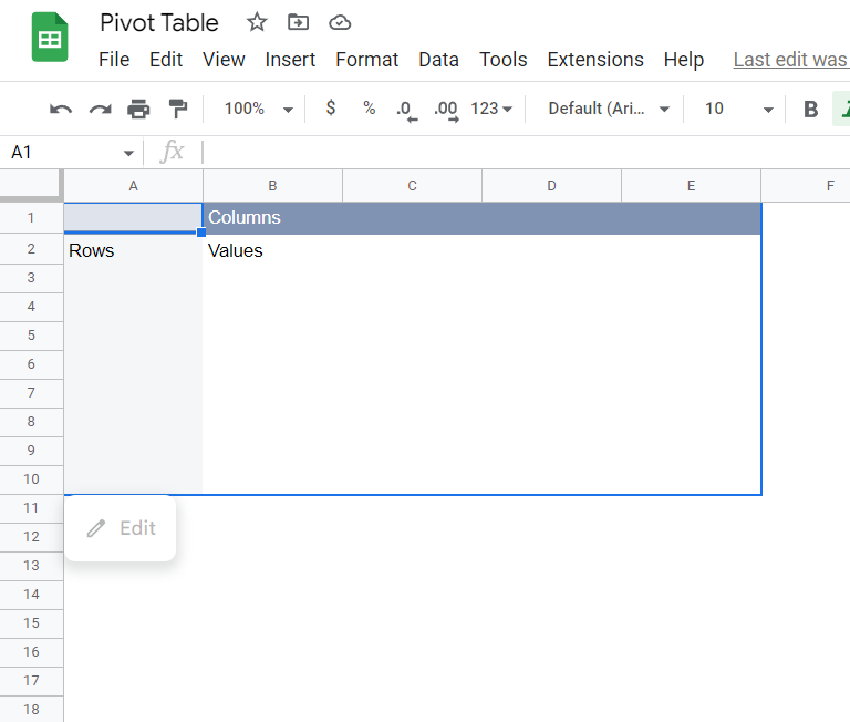
In screenshot 5, there are suggestions for creating tables; if you want to create your own version of the table with different aspects, you can add rows and columns with values.
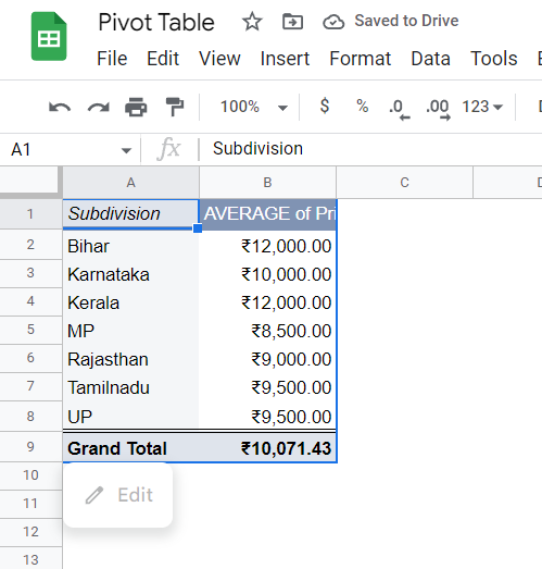
 Screenshot 5: Select “Average of Price per unit for each subdivision”
Screenshot 6 shows a table that was generated automatically by choosing from options.
 Screenshot 6: Pivot Table 1
4. Edit to obtain the required table
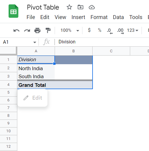
In order to create a pivot table, click the add from rows option. A drop-down menu containing various options from the data set will then appear; click any of them to build a table around it.
 Screenshot 7: Edit Pivot Table
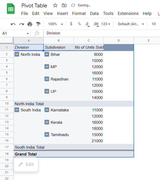
Similarly, you may add more rows by selecting the add option. In this instance, we’ve created a pivot table that includes sales information for air conditioners in North and South India, with the subdivisions’ divisions framed and listed separately. See screenshot 8.
 Screenshot 8: Pivot Table 2
5. Add values into pivot table
You can enter data into the values format using the values option, which will result in the creation of a new row and a total of figures. screenshot 9 can be followed.
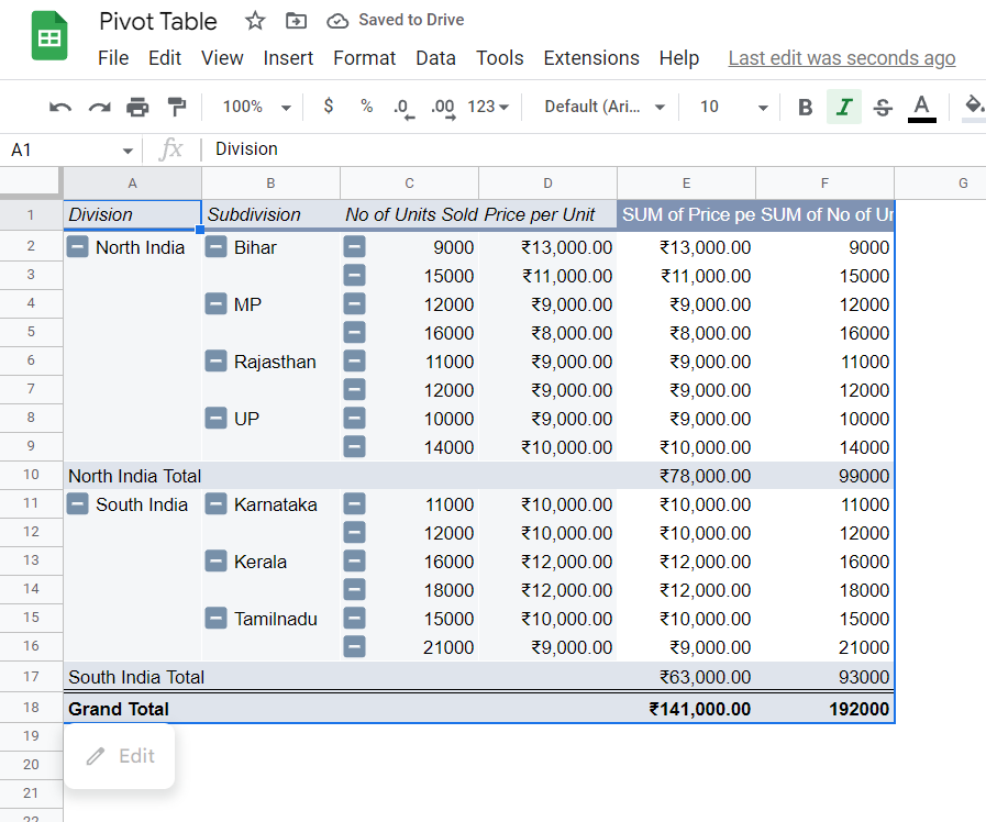 Screenshot 9: Pivot Table Example 3
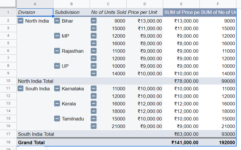
Included here an example link to the produced table here for your convenience- Pivot Table
Tags:
- #Google Spreadsheet,
- #Google Workspace